Adiabaticity, Stokes Phenomena, and Production Rates

Nonadiabatic production is controlled globally in complex time. A small real-time parameter such as $\lvert\omega'/\omega^2\rvert$ diagnoses local WKB quality, but the production exponent comes from complex zeros of $\omega^2$, and multiple turning-point pairs can interfere. A rate is justified only when the background supplies a long or repeated interval over which an extensive probability can be divided by time or volume.

Required background. Particle Creation in Time-Dependent Backgrounds supplies $\alpha$ and $\beta$; WKB and Eikonal Methods and Turning-Point Matching supplies local connection formulas; Laplace Method and Steepest Descent supplies saddle contours.

Helpful background. Stationary Phase, Coalescing Saddles, and Stokes Geometry supplies uniformization; Asymptotic Scales, Remainders, Uniformity, and Optimal Truncation supplies error language.

Dynamical WKB and turning points

Write a normalized mode as

$$v(t) = \frac{1}{\sqrt{2\omega(t)}} \left[ \alpha(t)e^{-i\theta(t)} +\beta(t)e^{+i\theta(t)} \right], \qquad \theta(t)=\int^t\omega(s)\,\mathrm ds.$$

One convenient phase convention gives

$$\dot\alpha = \frac{\dot\omega}{2\omega} e^{+2i\theta}\beta, \qquad \dot\beta = \frac{\dot\omega}{2\omega} e^{-2i\theta}\alpha,$$

and preserves $\lvert\alpha\rvert^2-\lvert\beta\rvert^2=1$. If $\beta(-\infty)=0$ and production is weak, the first iteration is

$$\beta(+\infty) \approx \int_{-\infty}^{\infty}\mathrm dt\, \frac{\dot\omega}{2\omega} \exp\!\left[-2i\int^t\omega(s)\,\mathrm ds\right].$$

Contour deformation shows that complex zeros of $\omega(t)^2$ and associated branch cuts control the exponentially small result. The local adiabaticity parameter

$$\epsilon(t) = \left\lvert \frac{\dot\omega}{\omega^2} \right\rvert$$

does not encode which saddles connect to the physical contour or how their phases interfere.

For isolated relevant turning points $t_p$, a semiclassical result has the structure

$$\beta \sim \sum_p \mathcal C_p \exp\!\left[ -2i\int^{t_p}\omega(t)\,\mathrm dt \right],$$

where $\mathcal C_p$ contains connection phases and prefactors. Production is $\lvert\beta\rvert^2$, so the sum must be formed before taking the modulus squared.

First application: a Sauter pulse

For a charged scalar in a homogeneous electric pulse, choose

$$A_\parallel(t) = -ET\tanh\frac{t}{T}, \qquad \omega_{\mathbf k}^2(t) = m_\perp^2 +\left[ k_\parallel-qA_\parallel(t) \right]^2,$$

with $m_\perp^2=m^2+k_\perp^2$. Complex turning points satisfy

$$k_\parallel+qET\tanh\frac{t_p}{T} = \pm i m_\perp.$$

The pair closest to the real axis gives the leading tunneling action

$$K_{\mathbf k} = \left\lvert \int_{t_-}^{t_+}\omega_{\mathbf k}(t)\,\mathrm dt \right\rvert, \qquad n_{\mathbf k}\sim e^{-2K_{\mathbf k}}$$

when it is isolated and the prefactor is controlled. The exact Sauter solution supplies an independent check.

Now replace one pulse by two separated pulses. Two turning-point pairs can contribute:

$$n_{\mathbf k} \approx e^{-2K_1} +e^{-2K_2} +2e^{-(K_1+K_2)} \cos\!\left(2\Theta_{\mathbf k}+\varphi\right).$$

The interference phase $\Theta_{\mathbf k}$ is accumulated between the pairs. Dumlu and Dunne show that this Stokes interference explains oscillatory Schwinger spectra in structured pulses Dumlu and Dunne 2010, pp. 250402-1–250402-4, eqs. (7)–(8).

Rates, prefactors, and uniform errors

The exponent is not the whole answer. Spin, degeneracy, connection phases, fluctuation determinants, and phase-space measures enter the prefactor. When turning points coalesce, isolated Airy connections fail and must be replaced by a uniform approximation. When several saddles have comparable action, omitting one is an $O(1)$ relative error near destructive interference.

A finite pulse gives a probability or produced density. Calling it a rate requires an extensive limit, for example a field that remains nearly constant for time $T_{\mathrm{obs}}$ with

$$-\log P_{\mathrm{vac}} \sim VT_{\mathrm{obs}}\,\Gamma$$

and edge corrections small compared with $VT_{\mathrm{obs}}$. A single-pulse yield divided by its arbitrary width is not a universal rate.

Adversarial local-adiabaticity test

Construct two profiles with the same maximum $\epsilon(t)$ on the real axis: a single pulse and a separated double pulse. The local diagnostic can be nearly identical, while the second spectrum has interference zeros and maxima. A formula $n\sim e^{-C/\epsilon_{\max}}$ cannot recover them.

The strongest surviving statement from $\epsilon\ll1$ alone is that the real-axis WKB expansion is locally accurate away from turning points. A production estimate additionally requires the analytic continuation, relevant saddle set, Stokes multipliers, prefactors, and a comparison with an exact or converged benchmark.

Construction and failure maps

The construction map places Stokes analysis after the frequency profile and asymptotic state are specified, and before a production exponent is interpreted as a number or rate.

Semiclassical production requires the relevant complex saddle set, connection data, prefactor, and asymptotic energy check; the map is schematic and not to scale.

The failure map targets two abuses: a local adiabaticity number is not a global production rate, and a finite-pulse yield is not an asymptotic rate.

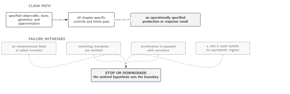
The saddle topology and asymptotic regime set the claim domain; one real-time adiabaticity parameter cannot replace them. Schematic and not to scale.

Compare the Stokes row in Domain and failure conditions. Report the analytic continuation used, turning points, contour, Stokes graph, action, prefactor, interference phase, uniformity parameter, asymptotic normalization, and independent benchmark.

Check your understanding

Why must the saddle amplitudes be summed before squaring?

Solution

Quantum alternatives add at the amplitude level. For $\beta=\beta_1+\beta_2$,

$$\lvert\beta\rvert^2 = \lvert\beta_1\rvert^2 +\lvert\beta_2\rvert^2 +2\operatorname{Re}(\beta_1\beta_2^*).$$

The last term produces enhancement or suppression and can be as large as the individual terms. Squaring each saddle first discards the Stokes interference.

Parametric-Oscillator and Solvable Production Benchmarks supplies exact fixtures. General asymptotic analysis remains in Volume I, adiabatic state regularity in Chapter 2, and adiabatic subtraction in Chapter 7.

References

• Michael V. Berry and Kenneth E. Mount, “Semiclassical Approximations in Wave Mechanics,” Reports on Progress in Physics 35 (1972), 315–397, DOI.
• Cesim K. Dumlu and Gerald V. Dunne, “The Stokes Phenomenon and Schwinger Vacuum Pair Production in Time-Dependent Laser Pulses,” Physical Review Letters 104 (2010), 250402, DOI, arXiv:1004.2509.
• Gerald V. Dunne, “Heisenberg–Euler Effective Lagrangians: Basics and Extensions,” in From Fields to Strings, World Scientific (2005), 445–522, DOI, arXiv:hep-th/0406216.