Inflationary Perturbations and Gauge-Invariant Variables

Cosmological perturbations contain both physical fluctuations and changes of coordinates. Gauge-invariant combinations remove infinitesimal redundancy once the background, transformation convention, and boundary conditions are fixed; they do not by themselves remove large transformations or turn a coordinate-space field into a fully relational observable.

Required background. Background symmetry breaking and decoupling supplies the clock and ADM constraints, while FLRW fields and mode quantization supplies the background decomposition.

Helpful background. Spinor and gauge fields in FLRW shows how the inventory changes for other spins; relational gravitational observables explains the further completion needed beyond linear gauge invariance.

Scalar transformations and invariant combinations

In conformal time, decompose the scalar metric sector as

$$ds^2=a^2\left[(1+2A)d\eta^2-2\partial_iB\,d\eta\,dx^i -\bigl((1+2C)\delta_{ij}+2\partial_i\partial_jE\bigr)dx^i dx^j\right].$$

Adopt the passive change $\eta\mapsto\eta+T$ and $x^i\mapsto x^i+\partial^iL$. With $\mathcal H=a'/a$,

$$\begin{aligned} A&\mapsto A-T'-\mathcal HT,& B&\mapsto B+T-L',\\ C&\mapsto C-\mathcal HT,& E&\mapsto E-L,\\ \delta\phi&\mapsto\delta\phi-\phi_0'T. \end{aligned}$$

Writing $q=B-E'$, invariant representatives are

$$\Phi=A+q'+\mathcal Hq,\qquad \Psi=-C-\mathcal Hq,\qquad \delta\phi_{\rm gi}=\delta\phi+\phi_0'q.$$

The comoving curvature perturbation in this chapter is

$$\zeta=C-\frac{\mathcal H}{\phi_0'}\delta\phi.$$

It equals $C$ in comoving gauge and $-\mathcal H\delta\phi/\phi_0'$ in spatially flat gauge. This sign agrees with $h_{ij}=a^2e^{2\zeta}\delta_{ij}$ and with $\zeta=-H\pi$ for the Stückelberg convention used in the previous page. Equivalent notations with $1-2\psi$ in the spatial metric have $C=-\psi$; translating that sign is essential.

The construction and the role of the scalar constraints are developed in Mukhanov, Feldman, and Brandenberger 1992, §§2–5, pp. 209–250.

Scalars, vectors, and tensors

The scalar lapse and shift equations relate $A$, $B$, $C$, $E$, and matter perturbations. For a canonical single field, one scalar combination remains dynamical. Vector metric perturbations have no propagating source-free mode in the minimal scalar model and decay after their constraint is imposed. The transverse-traceless tensor $\gamma_{ij}$ is already invariant under linear scalar and vector transformations and carries two helicities.

This counting is a statement about the quadratic theory around the chosen background. At second order, products of first-order scalar transformations source objects with vector and tensor index structure, so “the tensor perturbation” itself acquires a nonlinear gauge correction. One must either construct the second-order invariant combination or calculate a final quantity in two complete gauges. Similarly, adding a gauge field, a fluid with vorticity, or several scalar clocks changes the constraint sources and can make vector or entropy modes dynamical. The linear single-clock inventory cannot simply be copied into those systems.

As a first application, compare Newtonian gauge, $B=E=0$, with comoving gauge, $\delta\phi=E=0$. In Newtonian gauge the invariant potentials are simply $\Phi=A$ and $\Psi=-C$; in comoving gauge $\zeta=C$. Solving the constraint equations and translating through the invariant combinations gives the same $\zeta$ evolution in both gauges. Agreement requires carrying the lapse, shift, and any boundary term through the calculation, rather than identifying two gauge-fixed fields by name.

The structure map places the gauge-invariant reduction before canonical normalization and state selection.

Infinitesimal gauge transformations first organize perturbations into invariant combinations; constraints then reduce the minimal single-clock system to one scalar mode and two tensor helicities. Schematic; not to scale.

Residual transformations and observable scope

Definitions involving $\nabla^{-2}$ assume boundary conditions and exclude its zero mode. A spatially homogeneous time reparameterization can preserve common gauge conditions while shifting the apparent long-wavelength perturbation. Large dilations can similarly act nontrivially at the boundary. The adversarial test is therefore a zero-momentum transformation: determine whether it is pure redundancy for the chosen boundary conditions, an adiabatic physical mode, or a change of the relational frame.

Linear Bardeen variables are sufficient for local evolution at first order, but a finite-region measurement needs clocks, rods, or an asymptotic prescription. See the chapter’s domain and failure conditions. The validity map distinguishes ordinary gauge fixing from unresolved residual and relational questions.

A useful practical check is to construct a scalar from the perturbed intrinsic curvature of a slice selected by the clock, rather than from a coordinate component alone. Expanding that scalar in Newtonian and comoving gauges reproduces the same first-order $\zeta$ and reveals which second-order terms are part of the observable map. This also makes boundary assumptions visible: a clock slicing that fails where $\phi_0'=0$ cannot define a global relational observable there.

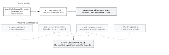
Gauge-invariant perturbation theory controls infinitesimal redundancy only after boundary and zero-mode conditions are fixed; large transformations and operational observables require additional data. Schematic; not to scale.

References

• Mukhanov, V. F., H. A. Feldman, and R. H. Brandenberger, “Theory of Cosmological Perturbations,” Physics Reports 215, 203–333 (1992), doi:10.1016/0370-1573(92)90044-Z.