Relative Cauchy Evolution and Background Response

Relative Cauchy evolution measures how an observable algebra responds when the background is changed inside a compact spacetime region. The comparison uses the time-slice property to identify the original and perturbed theories in the causal past and future of the change. For a metric perturbation, its first variation is generated by the stress tensor under the stated sign and normalization conventions; the construction is valid only while the perturbed background remains in the theory’s causal category.

Required background. Local Covariance, Isometries, and Background Embeddings supplies the comparison maps; Local Field Algebras, Causality, and the Time-Slice Property supplies their invertibility.

Helpful background. Coupling to Background Gauge Fields and Bundles gives nonmetric variations; Presymplectic Systems and the Covariant Phase-Space Ambiguity Map supplies the classical response.

Comparing two metrics through time slices

Let $(M,g)$ be globally hyperbolic and let $h_{\mu\nu}$ be a smooth compactly supported perturbation such that

$$g_h=g+h$$

is again a globally hyperbolic Lorentzian metric with the same orientation and time orientation. Choose globally hyperbolic neighborhoods $M_-$ and $M_+$ to the past and future of $\operatorname{supp}h$, each containing a Cauchy surface. They embed into both $(M,g)$ and $(M,g_h)$:

$$i_\pm:M_\pm\to(M,g), \qquad j_\pm:M_\pm\to(M,g_h).$$

Every induced algebra map is an isomorphism onto the full algebra by the time-slice property. With the convention that evolution crosses the perturbation from future data back to past data, define

$$\operatorname{rce}_M[h] = \mathcal A(i_-) \circ\mathcal A(j_-)^{-1} \circ\mathcal A(j_+) \circ\mathcal A(i_+)^{-1}.$$

This is an automorphism of $\mathcal A(M)$. Reversing the comparison order gives its inverse, so derivative signs must always be tied to the declared convention. Changing the auxiliary time-slice neighborhoods does not change the automorphism.

For a free scalar, the same construction can be seen at the level of solutions. If $P_h=P+\delta P+O(h^2)$, causal Møller maps compare solutions of $P\phi=0$ and $P_h\phi_h=0$. To first order their difference contains

$$E\,\delta P,$$

with retarded or advanced support selected on the corresponding side of the perturbation. This supplies a direct causal check on the algebraic definition.

Metric response and the stress tensor

For a differentiable theory, vary $h_{\mu\nu}$ in a compact region. In a representation where the renormalized stress tensor is defined, the derivative has the form

$$\left. \frac{\mathrm d}{\mathrm ds} \operatorname{rce}_M[sh](A) \right|_{s=0} = \frac{i}{2} \left[ \int_M T^{\mu\nu}h_{\mu\nu}\,\mathrm d\mathrm{vol}_g, A \right],$$

up to the sign fixed by whether the metric or inverse metric is varied and by the chosen direction of relative evolution. The invariant content is that the renormalized stress tensor generates infinitesimal metric response. Brunetti, Fredenhagen, and Verch establish this relation for the locally covariant framework Brunetti, Fredenhagen, and Verch 2003, §4.

This statement does not define the stress tensor’s finite renormalization by itself. Local curvature counterterms shift the renormalized tensor by conserved local terms. Chapter 7 classifies that freedom.

The same logic applies to other backgrounds. Varying a background gauge connection couples to a current; varying a mass profile couples to the corresponding local composite operator. Each response requires that the varied object be part of the background category and that the relevant composite field has been renormalized.

First application: a compact metric perturbation in a slab

Place $\operatorname{supp}h$ between Cauchy surfaces $\Sigma_-$ and $\Sigma_+$. An observable $A$ localized entirely to the causal complement of the perturbation has

$$\operatorname{rce}_M[h](A)=A$$

whenever causal propagation cannot connect its localization region to $\operatorname{supp}h$. For a scalar observable $\Phi(f)$ that can be influenced, the first variation follows by differentiating the perturbed equation:

$$P\,\delta\phi = -(\delta P)\phi, \qquad \delta\phi_{\mathrm{ret}} = -G_{\mathrm{ret}}(\delta P)\phi.$$

The support of $\delta\phi_{\mathrm{ret}}$ lies in the causal future of the metric perturbation. This is the response check: the algebraic automorphism and the differential-operator calculation must have the same causal support.

As an adversarial test, allow $h$ to reach a timelike boundary while holding the boundary condition fixed only symbolically. The perturbation can change the unit normal, the boundary form, or the admissible self-adjoint domain, so the maps $j_\pm$ need not compare the same theory. Alternatively, let $g+h$ cease to be globally hyperbolic. Then the time-slice isomorphisms used in the definition are unavailable. In either case, the formula must be restricted or replaced by a boundary-sensitive construction.

Construction and failure maps

The first schematic shows why relative Cauchy evolution is possible: causal dynamics and the time-slice property construct the algebra before the metric response is evaluated in any state.

Relative Cauchy evolution is an algebra automorphism built from past and future time slices; expectation-value response is a later, state-dependent step. Schematic and not to scale.

For the second schematic, inspect the global-hyperbolicity and boundary-flux witnesses. Either one can invalidate the comparison maps even when the formal first variation of $P$ exists.

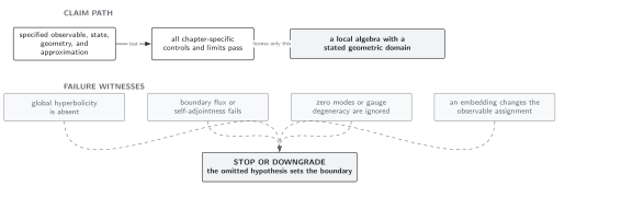
Stress-tensor response is licensed only for compact admissible background variations within a fixed theory; changed causal or boundary data require a restricted claim. Schematic and not to scale.

The chapter comparison appears under Domain and failure conditions. Here one must check compact support, persistence of global hyperbolicity, unchanged auxiliary background data, causal support of the response, and the renormalization convention for the generator.

Check your understanding

Why is compact support of $h_{\mu\nu}$ useful in the construction?

Solution

It leaves common past and future regions where $g_h=g$. Those regions can contain Cauchy surfaces and embed into both backgrounds, so their time-slice maps provide the canonical comparison. A perturbation extending to all times need not leave such common regions.

Stress-tensor renormalization is developed in Local Observables, Stress Tensors, and Anomalies; solving the mean metric equation belongs to Mean Semiclassical Backreaction. The theorem-level relation to dynamical locality remains in Volume XVI.

References

• Romeo Brunetti, Klaus Fredenhagen, and Rainer Verch, “The Generally Covariant Locality Principle—A New Paradigm for Local Quantum Field Theory,” Communications in Mathematical Physics 237 (2003), 31–68, DOI, arXiv:math-ph/0112041.
• Christopher J. Fewster and Rainer Verch, “Algebraic Quantum Field Theory in Curved Spacetimes,” in Advances in Algebraic Quantum Field Theory, Springer (2015), 125–189, DOI, arXiv:1504.00586, §4.
• Stefan Hollands and Robert M. Wald, “Quantum Fields in Curved Spacetime,” Physics Reports 574 (2015), 1–35, DOI, Open PDF, §4.