

Heat Kernels with Boundaries and Conical Singularities
A boundary or conical stratum changes the operator domain and the heat-kernel asymptotics. The resulting surface, corner, and tip coefficients are not optional decorations on the smooth bulk answer: they renormalize localized terms and can control determinant variations.
Required background. Heat Kernels and the Schwinger–DeWitt Expansion supplies the smooth short-time series, and Boundaries, Surface Counterterms, and Boundary Stress supplies the localized variational terms.
Helpful background. Replica Trick and Branched Geometries explains one use of cones; Timelike Boundaries, Self-Adjoint Extensions, and AdS Boundary Conditions explains Lorentzian boundary dynamics.
Elliptic boundary data
Section titled “Elliptic boundary data”For a scalar Laplace-type operator on a smooth Riemannian manifold with boundary, common local domains are
and
where and the sign of the extrinsic curvature are declared. Self-adjointness follows from the vanishing of the Green-form boundary term for compatible real ; ellipticity or strong ellipticity is an additional analytic requirement.
The traced heat kernel now has half-integer powers,
With Vassilevich’s inward-normal convention, a scalar gives
and the boundary part of is
for Robin, with for Dirichlet in this order and with following that same normal convention. The complete bundle formulas and normal conventions are given in Vassilevich 2003, Eqs. (2.14)–(2.17) and (5.18)–(5.33).
First application: Robin versus Dirichlet
Section titled “First application: Robin versus Dirichlet”Hold the bulk scalar operator fixed and switch from Robin to Dirichlet data. The bulk coefficients and the interior part of are unchanged. The first surface coefficient changes by
and the Robin parameter supplies the additional term at the next order. In four dimensions these coefficients generate boundary divergences at the corresponding mass dimensions after multiplication by the mass expansion. The necessary counterterms therefore include the boundary volume, extrinsic-curvature terms, and invariants involving .
This is the adversarial test required by the domain: a calculation that changes boundary conditions yet reports identical surface coefficients has silently reused the wrong spectrum. A calculation whose bulk coefficient changes has mixed a boundary effect into the differential expression.
A conical tip is not a smooth point
Section titled “A conical tip is not a smooth point”Near a two-dimensional cone,
the tip is singular unless . Even without a boundary, conical heat traces can contain nonstandard powers and logarithms. For the flat two-dimensional cone in the standard scalar case, the localized coefficient is
which vanishes at and behaves as for a small deficit Vassilevich 2003, § 6.2 and Eq. (6.7). Higher-dimensional products generate defect invariants on the codimension-two surface.
A smoothing prescription can be useful, but the limit must retain the integrated defect contribution. Simply substituting a distributional curvature into a smooth coefficient polynomial can create undefined products such as . Replica or entropy interpretations additionally require an analytic continuation in the cone angle and a declared treatment of edge and gauge modes; the heat coefficient alone is not an entropy theorem.
The structure map shows boundaries and cones as a change in the spectral problem, not as a correction applied after taking a smooth determinant.

Bulk, boundary, corner, and tip invariants enter at different powers of proper time and renormalize different localized terms. Schematic; not to scale.
Domain and failure conditions
Section titled “Domain and failure conditions”Local formulas require a self-adjoint strongly elliptic boundary problem and smooth boundary data. Corners, oblique conditions, spectral projectors, and general cones can introduce additional or nonlocal terms. See Domain and failure conditions.
The failure map distinguishes an undefined extension from a singular geometry. Choosing a self-adjoint extension does not smooth a cone; smoothing a cone does not choose boundary data on a physical wall.
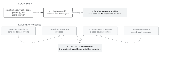
Surface coefficients follow from the operator domain, while tip coefficients follow from singular geometry and its regularization; each must be checked independently. Schematic; not to scale.
Related topics
Section titled “Related topics”Boundary stress and finite counterterms continue in Boundaries, Surface Counterterms, and Boundary Stress. Replica use continues in Replica Trick and Branched Geometries.