In-In Cosmological Correlators

Cosmological observations depend on expectation values in an initial state, not on amplitudes between independently chosen “in” and “out” vacua. The in-in, or closed-time-path, formalism evolves the ket forward and the bra backward to the same observation time, making normalization, causality, and reality visible order by order.

Required background. Gauge-invariant perturbations supplies the fields being measured; in-out versus in-in expectation values supplies the conceptual distinction; and closed-time-path generating functionals supplies doubled real-time evolution.

Helpful background. Initial density matrices and boundary EFT treats nonvacuum states, while unitarity, normalization, and largest-time identities supplies diagrammatic checks.

Closed evolution to a finite observation time

Let $H=H_0+H_I$ and let $Q_I(t)$ be an interaction-picture operator. For a pure state prepared in the asymptotic past,

$$\langle Q(t)\rangle= \left\langle \bar T\exp\!\left(i\int_{-\infty}^{t}dt'\,H_I(t')\right) Q_I(t) T\exp\!\left(-i\int_{-\infty}^{t}dt'\,H_I(t')\right) \right\rangle.$$

For a density matrix $\rho_0$, the bracket means a trace with $\rho_0$. The forward and backward branches share the same final field configuration before it is integrated over. Consequently

$$Z[J,J]=\operatorname{Tr}\rho_0=1$$

for a normalized state. This identity cancels vacuum bubbles and is stronger than dividing an in-out amplitude by a vacuum persistence amplitude.

At first order,

$$\delta\langle Q(t)\rangle =-i\int_{t_0}^{t}dt_1\, \langle[Q_I(t),H_I(t_1)]\rangle =i\int_{t_0}^{t}dt_1\, \langle[H_I(t_1),Q_I(t)]\rangle.$$

Iterating gives a nested-commutator expansion whose time limits are manifestly retarded. Weinberg derives this form and its late-time power counting in Weinberg 2005, §§II–IV, Eqs. (1)–(19).

Equivalently, contour perturbation theory uses four propagators $G^{ab}$ with $a,b\in\{+,-\}$. They are not independent: $G^{++}+G^{--}=G^{+-}+G^{-+}$. This identity encodes the cancellation that occurs when the two sources coincide. Rotating to center/difference variables turns the same matrix into retarded, advanced, and statistical functions, making causal response distinct from state fluctuations. Keeping this matrix structure intact is especially useful at loop order, where assigning an ordinary Feynman propagator to every internal line would compute the wrong object.

Tree-level three-point function

For a cubic interaction, the first contribution to a late-time scalar three-point function is

$$\langle\zeta_{\mathbf k_1}(t) \zeta_{\mathbf k_2}(t)\zeta_{\mathbf k_3}(t)\rangle' =-i\int_{t_0}^{t}dt_1\, \left\langle \left[\zeta_{\mathbf k_1}(t)\zeta_{\mathbf k_2}(t) \zeta_{\mathbf k_3}(t),H_I(t_1)\right] \right\rangle.$$

The prime removes $(2\pi)^3\delta^3(\mathbf k_1+\mathbf k_2+\mathbf k_3)$. Evaluating this commutator or summing the $+$ and $-$ contour vertices gives the same real result. A residual imaginary answer indicates a missing conjugate branch, an inconsistent $i\epsilon$, or an endpoint term.

The interaction Hamiltonian cannot always be obtained by writing $H_I=-L_I$: derivative interactions modify the canonical momenta, and the Legendre transform must be performed to the relevant order. At leading cubic order in many standard scalar examples the shortcut happens to hold after constraints are reduced, but it is not a general theorem.

The final observation time also remains finite until the calculation is assembled. Taking $t\to\infty$ inside separate branch integrals can create spurious divergences that cancel only in the commutator sum. A safe procedure combines the branches, renormalizes composite insertions, and only then takes a late-time limit whose convergence or secular behavior is demonstrated.

The structure map shows the doubled contour connecting a specified initial state to a finite-time observable.

The in-in contour evolves the ket and bra to one observation time; summing both branches enforces normalization, causal commutators, and reality. Schematic; not to scale.

Unitarity and free-theory checks

Set $H_I=0$: every correction must vanish and the result must reduce to the chosen free-state correlator. Next set $J_+=J_-$ in the generating functional: all connected vacuum contributions must cancel exactly. Finally place a latest-time vertex beyond every measured insertion; the sum over its two branch assignments must vanish. These are algebraic checks before any momentum integral is trusted.

The same contour computes unequal-time or composite observables, but those require their own ordering and renormalization. See the chapter’s domain and failure conditions. The validity map emphasizes that an in-out amplitude, a single contour branch, or an unnormalized initial state cannot substitute for this construction.

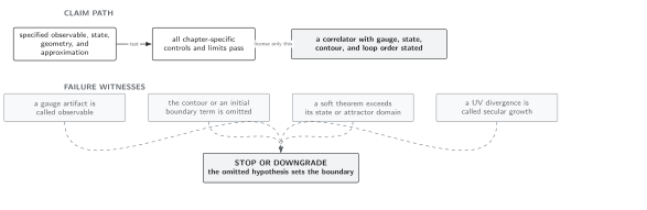
Normalized in-in predictions must pass the free limit, $Z[J,J]=1$, reality, and largest-time cancellation before physical interpretation. Schematic; not to scale.

References

• Weinberg, S., “Quantum Contributions to Cosmological Correlations,” Physical Review D 72, 043514 (2005), doi:10.1103/PhysRevD.72.043514.