Green Operators, Causal Propagators, and State-Dependent Two-Point Functions

The field equation fixes causal response but not quantum fluctuations. On a globally hyperbolic spacetime, a normally hyperbolic operator has unique retarded and advanced Green operators. Their difference is a homogeneous causal propagator and fixes the commutator. A Wightman or Feynman two-point function additionally encodes a quantum state, so it changes when the state changes even though the equation and causal response remain fixed.

Required background. Curved Spacetimes, Cauchy Surfaces, and Global Hyperbolicity supplies the causal hypotheses; Fundamental Solutions and Green Operators supplies distributional inverses; Hyperbolic Equations and Causal Propagators fixes the site’s propagator convention.

Helpful background. Scalar Propagators, Ordered Correlators, and Sources gives the flat-space dictionary; Singular Support and Wavefront Sets and Distributional Kernels on Manifolds prepare the microlocal refinement.

Retarded, advanced, and causal Green operators

Let $P:\Gamma(E)\to\Gamma(E)$ be a formally self-adjoint normally hyperbolic operator on a globally hyperbolic spacetime. For $f\in\Gamma_0(E)$, the retarded and advanced Green operators satisfy

$$PG_{\mathrm{ret/adv}}f=f, \qquad G_{\mathrm{ret/adv}}Pf=f,$$

with support conditions

$$\operatorname{supp}G_{\mathrm{ret}}f \subset J^+(\operatorname{supp}f), \qquad \operatorname{supp}G_{\mathrm{adv}}f \subset J^-(\operatorname{supp}f).$$

Global hyperbolicity is what turns the local fundamental solution into a unique global operator with these support properties Bär, Ginoux, and Pfäffle 2007, Theorem 3.3.1 and Corollary 3.4.3.

This chapter follows the established Volume I convention

$$E \equiv G_{\mathrm{ret}}-G_{\mathrm{adv}}.$$

Then $PE=EP=0$ on compactly supported test sections. For a real bosonic field,

$$[\Phi(f),\Phi(h)] = -iE(f,h)\,\mathbf1, \qquad E(f,h) = \int_M f\,Eh\,\mathrm d\mathrm{vol}_g.$$

Many texts instead write $\Delta=G_{\mathrm{adv}}-G_{\mathrm{ret}}=-E$, in which case the same relation is $[\Phi(f),\Phi(h)]=i\Delta(f,h)\mathbf1$. The physics is unchanged only when the definitions and commutator sign are translated together.

The retarded response to a classical source $J$ is

$$\delta\phi=G_{\mathrm{ret}}J.$$

It depends on $P$ and the causal problem, not on a choice of vacuum or density matrix.

State-dependent two-point functions

A state $\omega$ supplies the Wightman two-point distribution

$$W_\omega(f,h) \equiv \omega\!\left(\Phi(f)\Phi(h)\right).$$

For a quasifree scalar state it must satisfy the field equation in both entries, positivity,

$$W_\omega(\bar f,f)\ge0,$$

and the fixed antisymmetric part

$$W_\omega(f,h)-W_\omega(h,f) = -iE(f,h).$$

The symmetric part is state data. It controls fluctuations and detector excitation, while the antisymmetric part is fixed by the causal propagator.

On a spacetime with a suitable time function, the time-ordered distribution is assembled from the same state,

$$W_{\mathrm T}(x,y) = \theta(t_x-t_y)W_\omega(x,y) +\theta(t_y-t_x)W_\omega(y,x).$$

Depending on the convention for factors of $i$, a “Feynman propagator” may mean $W_{\mathrm T}$ or a multiple of it. Its wavefront prescription and inhomogeneous equation must therefore be stated. Unlike $G_{\mathrm{ret}}$, it is not characterized by future support. Chapter 2 imposes the Hadamard ultraviolet condition needed for local composite operators.

Distribution	Fixed by $P$ and causal domain?	Requires a state?	Defining information
$G_{\mathrm{ret}}$	Yes	No	Inverse with future support
$G_{\mathrm{adv}}$	Yes	No	Inverse with past support
$E=G_{\mathrm{ret}}-G_{\mathrm{adv}}$	Yes	No	Homogeneous causal propagator and commutator
$W_\omega$	No	Yes	Positive bisolution with fixed antisymmetric part
$W_{\mathrm T}$	No	Yes	Time ordering of $W_\omega$

First application: an ultrastatic scalar

Take

$$M=\mathbb R\times\Sigma, \qquad P=\partial_t^2+A,$$

where $A$ is a positive self-adjoint spatial operator on $L^2(\Sigma)$. Functional calculus gives the retarded kernel

$$G_{\mathrm{ret}}(t,t') = \theta(t-t') \frac{\sin\!\left(A^{1/2}(t-t')\right)}{A^{1/2}},$$

and

$$E(t,t') = \frac{\sin\!\left(A^{1/2}(t-t')\right)}{A^{1/2}}.$$

The distributional derivative of the step function supplies the unit jump required by $PG_{\mathrm{ret}}=\mathbf1$. If $A$ has a zero mode, the ratio is understood by its continuous limit, $\sin(\sqrt\lambda\,\tau)/\sqrt\lambda\to\tau$; whether that mode admits a stationary ground state is a separate infrared question.

For strictly positive $A$, the ultrastatic ground-state two-point function is

$$W_0(t,t') = \frac{e^{-iA^{1/2}(t-t')}}{2A^{1/2}}.$$

Its antisymmetric part is

$$W_0(t,t')-W_0(t',t) = -iE(t,t'),$$

as required. Thermal and squeezed quasifree states replace the symmetric covariance but preserve this difference.

Adversarial state replacement

Keep $P$, the spacetime, and all boundary conditions fixed, and replace $W_\omega$ by

$$W_{\omega'}=W_\omega+H,$$

where $H$ is a real symmetric bisolution chosen so that positivity is preserved. Then

$$P_xH=P_yH=0, \qquad H(x,y)=H(y,x).$$

The Wightman and time-ordered functions change. Particle interpretations, fluctuation amplitudes, and detector transition probabilities can change as well. But $G_{\mathrm{ret}}$, $G_{\mathrm{adv}}$, $E$, and the commutator do not change, because they are fixed before a state is chosen.

This test catches a common category error: a retarded response is not a vacuum correlator. Conversely, knowing the commutator does not determine the symmetric covariance. A candidate two-point function must pass the field equation, positivity, commutator, and—when ultraviolet composites are intended—Hadamard tests separately.

Construction and failure maps

The first map separates the Green-hyperbolic operator from the later state-dependent box. For this page, $G_{\mathrm{ret}}$, $G_{\mathrm{adv}}$, and $E$ are fixed before $W_\omega$ is supplied.

Causal Green operators belong to the dynamical construction, whereas the symmetric two-point covariance belongs to a chosen state; the map is schematic and not to scale.

In the failure map, global hyperbolicity tests existence and uniqueness, while the commutator-sign checkpoint tests convention consistency. Positivity and Hadamard form are additional state checks, not properties of $G_{\mathrm{ret}}$.

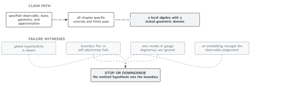
Each distribution is licensed by its own equation, support, antisymmetry, and positivity conditions; changing a state must not change causal response. Schematic and not to scale.

See Domain and failure conditions. Here the decisive checks are the two inverse identities, future or past support, $E=G_{\mathrm{ret}}-G_{\mathrm{adv}}$, the commutator $-iE$, bisolution property, and state positivity.

Check your understanding

Why does adding a symmetric bisolution leave the commutator unchanged?

Solution

For $W'=W+H$ with $H(f,h)=H(h,f)$,

$$W'(f,h)-W'(h,f) = W(f,h)-W(h,f).$$

Thus the antisymmetric part remains $-iE(f,h)$. Because $H$ is a bisolution, the field equation also remains satisfied. Positivity is not automatic and must still be checked.

The causal propagator next becomes a symplectic pairing in Covariant Symplectic Structure and Conserved Inner Products. State construction, Hadamard wavefront sets, and ultraviolet admissibility belong to States, Hadamard Structure, and Microlocal Control.

References

• Christian Bär, Nicolas Ginoux, and Frank Pfäffle, Wave Equations on Lorentzian Manifolds and Quantization, European Mathematical Society (2007), DOI, Open PDF, Chapters 3–4.
• Marco Benini, Claudio Dappiaggi, and Thomas-Paul Hack, “Quantum Field Theory on Curved Backgrounds: A Primer,” International Journal of Modern Physics A 28 (2013), 1330023, DOI, arXiv:1306.0527, §§2–3.
• Stefan Hollands and Robert M. Wald, “Quantum Fields in Curved Spacetime,” Physics Reports 574 (2015), 1–35, DOI, Open PDF, §2.