Euclidean Periodicity, KMS Structure, and Horizon Thermality

Euclidean regularity, Lorentzian KMS analyticity, and detector detailed balance coincide for a suitable stationary horizon state, but none is a substitute for specifying that state. The conical argument fixes a period from a nonextremal static metric; turning that period into quantum thermality requires a valid analytic continuation and a horizon-regular Lorentzian two-point function.

Required background. Surface gravity and redshift fixes the Killing normalization; ground and KMS state selection supplies curved-space states; and thermal density operators and the KMS condition gives the algebraic definition.

Helpful background. Modular KMS correlators, accelerated detectors, the Bisognano–Wichmann theorem, and complete passivity provide complementary operational and structural formulations.

Conical regularity and KMS analyticity

Near a nonextremal static horizon, introduce proper distance $\rho$ so that

$$ds^2=(\kappa\rho)^2dt^2-d\rho^2-h_{AB}dy^Ady^B+O(\rho^2).$$

After $t=-i\tau$, the two-dimensional normal metric is

$$ds_E^2=d\rho^2+\kappa^2\rho^2d\tau^2.$$

It is smooth at $\rho=0$ only if

$$\tau\sim\tau+\beta_H, \qquad \beta_H=\frac{2\pi}{\kappa}.$$

Any other period produces a conical defect. The argument assumes a real, positive Euclidean section and a simple horizon zero. It says nothing by itself about collapse preparation or outward flux.

For a state $\omega$ stationary under Killing evolution $\alpha_t$, the KMS condition at inverse temperature $\beta$ requires, for suitable observables $A,B$, a function analytic in $0<\operatorname{Im}z<\beta$ whose boundary values obey

$$F_{A,B}(t)=\omega(A\alpha_t(B)), \qquad F_{A,B}(t+i\beta)=\omega(\alpha_t(B)A).$$

A Euclidean Green function periodic with $\beta_H$ that analytically continues to a Hadamard, horizon-regular Lorentzian state yields this KMS relation. Restricted to one static wedge, the Hartle–Hawking–Israel state has precisely that temperature under the hypotheses of the bifurcate-horizon theorem (Kay and Wald 1991, §§ 5–7).

A stationary detector of energy gap $\Omega>0$ then obeys detailed balance

$$\frac{\dot{\mathcal F}(+\Omega)} {\dot{\mathcal F}(-\Omega)} =e^{-\beta_{\rm loc}\Omega}, \qquad \beta_{\rm loc}=\beta_H\sqrt{\chi^2}.$$

This is a response ratio along a specified worldline. In a Hartle–Hawking equilibrium state, incoming and outgoing thermal fluxes can cancel even though the detector is thermal.

The structure map locates the KMS result in the near-horizon box, downstream of the stationary state and upstream of any scattering or net-flux statement.

Euclidean/KMS thermality in the controlled horizon construction. The diagram is schematic and not to scale; detailed balance is not an asymptotic luminosity.

The failure map highlights the category error of calling a KMS response an outward flux. It also stops an analytic-continuation argument when no real regular Euclidean section or Lorentzian state is available.

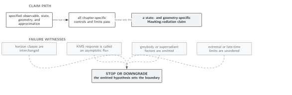
Failure boundary for horizon thermality. This schematic, not-to-scale map licenses only the geometric period, KMS state, detector response, or flux that has independently passed its defining test.

Application: matching the Euclidean and Lorentzian periods

For Euclidean Schwarzschild,

$$f(r)=1-\frac{2M}{r}, \qquad \kappa=\frac{1}{4M},$$

and the near-horizon plane is smooth for $\beta_H=8\pi M$. Constructing the Euclidean Green function with this period and analytically continuing its time arguments gives a Lorentzian two-point function periodic in imaginary Killing time in the KMS sense. It is regular across both future and past horizons in the maximally extended geometry and corresponds to thermal equilibrium, not the one-sided collapse flux.

For a nonstationary collapse metric there is no global Killing time to continue and no fixed Euclidean period. A late-time local temperature may emerge from ray tracing or detector response, but it is not derived by removing a global cone. For rotating horizons, regularity involves the horizon generator $\chi=\partial_t+\Omega_H\partial_\varphi$ and a joint thermal-angular identification; a naive real periodicity in $t$ alone ignores the chemical potential and may fail to define a regular bosonic state.

Domain and failure conditions

Use the chapter domain and failure-conditions table. Euclidean smoothness assumes a nonextremal stationary analytic section; KMS thermality additionally assumes a positive, Hadamard Lorentzian state under the normalized Killing flow. These license the period and detailed-balance ratio, respectively. Absence of stationarity or analytic continuation downgrades the result to local geometric peeling or detector evidence; rotation requires the combined generator and may face a state-existence obstruction. No KMS result alone licenses a nonzero net flux.

Exercise

Why does a Hartle–Hawking detector response coexist with zero net energy flux at infinity?

Solution

KMS detailed balance describes the ratio of excitation and de-excitation probabilities in a thermal bath. The Hartle–Hawking state contains both outgoing and incoming thermal sectors at the same temperature. Their asymptotic energy fluxes cancel in equilibrium even though either sector produces a thermal detector response.

Handoff

The next page defines the standard Boulware, Hartle–Hawking, and Unruh states by their horizon regularity and incoming/outgoing mode populations before any greybody calculation is performed.

References

• Gibbons, G. W., and Stephen W. Hawking. “Cosmological Event Horizons, Thermodynamics, and Particle Creation.” Physical Review D 15 (1977): 2738–2751. doi:10.1103/PhysRevD.15.2738.
• Hartle, James B., and Stephen W. Hawking. “Path-Integral Derivation of Black-Hole Radiance.” Physical Review D 13 (1976): 2188–2203. doi:10.1103/PhysRevD.13.2188.
• Kay, Bernard S., and Robert M. Wald. “Theorems on the Uniqueness and Thermal Properties of Stationary, Nonsingular, Quasifree States on Spacetimes with a Bifurcate Killing Horizon.” Physics Reports 207 (1991): 49–136. doi:10.1016/0370-1573(91)90015-E.